Modeling reinforcement learning (Part II): Maximum likelihood estimation
This post is the second in a series to describe how to fit a reinforcement learning model to data collected from human participants. Using example data from Speekenbrink and Konstantinidis (2015), we will go through all the steps in defining the model, estimating its parameters, and doing inference and model comparison.
In this post, we will use data from Speekenbrink and Konstantinidis (2015) to estimate the parameters of the Kalman filter with softmax model. We use this relatively simple model to introduce some important concepts such as the likelihood function, maximum likelihood estimation, numerical optimization, and discuss issues such as parameter identifiability. We also briefly cover estimating the Kalman filter + UCB model, but keep estimating the model with Thompson sampling for the next post. This post turned out rather long, but I decided to keep it as a single post rather than split it into separate ones.
The data
I have made the data from Speekenbrink and Konstantinidis (2015) available on GitHub. You can load it into R directly from there as follows:
dat <- read.csv("https://github.com/speekenbrink-lab/data/raw/master/Speekenbrink_Konstantinidis_2015.csv")
First, let’s have a look at the data:
head(dat)
##   cond id id2 seed trial deck payoff       rt block age gender
## 1  nts  1   1    1     1    2      2 1977.117     1  21 female
## 2  nts  1   1    1     2    2      0 3171.249     1  21 female
## 3  nts  1   1    1     3    2      1 2323.209     1  21 female
## 4  nts  1   1    1     4    2      6 2179.149     1  21 female
## 5  nts  1   1    1     5    2     14 2226.976     1  21 female
## 6  nts  1   1    1     6    2     13 2442.985     1  21 female
We can see that the dataset contains 11 variables. These are
condrefers to the condition (ntn = no trend, non-stable volatility, nts = no trend, stable volatility, tn = trend, non-stable volatility, ts = trend, stable volatility)id: participant id within a conditionid2: unique participant ID (more useful thanid)seed: particular random seed used to generate the mean rewardstrial: trial number, from 1 to 200deck: id of chosen bandit (the term “deck” is a reference to the Iowa gambling task)payoffreward obtained by choosingdeckontrialrt: reaction time in millisecondsblock: divides thetrialinto four blocks of 50 trials eachage: participant age in yearsgender: male or female (yes, this is certainly too restrictive and we now always include at least the options “other” and “prefer not to say” as well)
We’ll be mainly interested in modelling people’s deck choice as a
function of their experienced rewards. At a minimum, we might expect
people to try each option at least once, but this isn’t the case. If you
run e.g. with(dat,ftable(id2,deck)), you can see that participant with
id2 == 1 only chose option 2 throughout the whole experiment, never
exploring any of the other options at all (we ignored the data from this
participant in the paper).
For the purpose of this blog post, we will fit the model to the data of
a single participant, and I’ve (somewhat arbitrarily) chosen participant
with id2 == 4:
tdat <- subset(dat,id2==4)
Maximum likelihood estimation
Generally, cognitive models provide probabilistic predictions, assigning at each time point a probability to the relevant observable behaviour. In our case, we want to predict people’s choices Ct at each time t from what they have experienced up to that time in the task. In a bandit task, their experience consists of their previous choices C1 : (t − 1) = (C1, …, Ct − 1) and the associated rewards R1 : (t − 1) = (R1, …, Rt − 1). So the models should predict, on each trial t, the probability of choosing each option, conditionally upon the experience up to that point. More formally, this can be expressed as:
P(Ct|C1 : (t − 1), R1 : (t − 1), θ),
where θ are the model parameters. As we saw in the previous post, the softmax and Thompson sampling strategies directly provide these probabilities. The UCB strategy on the other hand is deterministic, so we’ll need to make some changes to provide probabilistic predictions (more about that later).
The basic idea of maximum likelihood estimation is to estimate parameters by finding those parameter values which assign the highest probability to the observed data. So, we will look for the values of the parameters θ which assign the highest probability to the choices that people made.
Fitting the Kalman filter + softmax model
In the previous post, we looked at three Bayesian RL models, which were all based on the Kalman filter, but used different choice rules.
Here is our function from the previous post to run the Kalman filter:
kalman_filter <- function(choice, reward, noption, mu0, sigma0_sq, sigma_xi_sq, sigma_epsilon_sq) {
  nt <- length(choice)
  no <- noption
  m <- matrix(mu0,ncol=no,nrow=nt+1)
  v <- matrix(sigma0_sq,ncol=no,nrow=nt+1)
  for(t in 1:nt) {
    kt <- rep(0,no)
    kt[choice[t]] <- (v[t,choice[t]] + sigma_xi_sq)/(v[t,choice[t]] + sigma_xi_sq + sigma_epsilon_sq)
    m[t+1,] <- m[t,] + kt*(reward[t] - m[t,])
    v[t+1,] <- (1-kt)*(v[t,] + sigma_xi_sq)
  }
  return(list(m=m,v=v))
}
Recall that softmax choice rule only uses the estimated mean rewards mt, and defines the probability of choosing an option as \(P(C_t = i|C_{0:(t-1)},R_{0:(t-1)},\theta) = \frac{\exp(\gamma m_{t,i})}{\sum_{j=1}^4 \exp(\gamma m_{t,j})}\)
Rather than simulating such choices, as we did in the last post, we now define a function which calculates the probability of choosing each option:
softmax_choice_prob <- function(m,gamma) {
  prob <- exp(gamma*m)
  prob <- prob/rowSums(prob) # normalize
  return(prob)
}
Assuming only γ is unknown
As an easy example, let’s start by assuming that we know the parameters of the Kalman filter. We then have one unknown parameter left: γ for the softmax choice rule. We will first inspect the likelihood function for a reasonable range of values of γ. Using a fixed set of possible parameter values, computing the likelihood for each, and then picking the value of the parameter with the highest likelihood, is a procedure known as grid search. This is straightforward to implement, although when the spacing between the evaluated points is coarse, it lacks precision. We therefore use the grid search procedure mainly for illustrative purposes, and then turn to more fine-grained numerical optimization routines in R to obtain the maximum likelihood estimate of this parameter.
To get started, we can define the likelihood function for γ as follows:
\[\begin{align} L(\gamma|C_{1:200},R_{1:200}) &= P(C_{1:200}|R_{1:200},\gamma) \\ &= P(C_{1}|\gamma) \times P(C_{2}|\gamma,R_{1},C_{1}) \times \ldots \times P(C_{200}|\gamma,C_{1:199},R_{1:199}) \\ &= \prod_{t=1}^T P(C_t|C_{0:(t-1)},R_{0:(t-1)},\gamma) \end{align}\]where on the last line, we define $C_0 = R_0 = \emptyset$ as null/empty values for convenient notation, so that for trial t = 1, we end up with P(C1|C0, R0, θ) = P(C1|θ).
Some quick comments: Firstly, here we have used the chain rule of probability to state the joint probability of all choices as the product of a number of conditional probabilities (where each choice depends on all previous choices and observed rewards). There are other ways to write the likelihood, but this version makes sense and corresponds to the order in which participants receive the information. Secondly, on the left hand side, we define the likelihood function L for γ conditional on the choices Ct and rewards Rt, while on the right hand side, we have the probability of the choices conditional on the rewards and the parameter γ. The reason for introducing the likelihood as a separate function, rather than a probability, is that having run the experiment, we can treat the observed data as given, or “fixed”. In estimation, we can then vary the parameter γ and get different values of the probability of the data. As a function of γ, the left hand side not a probability density function (i.e., when integrating the right hand side over all possible values of γ, the result is generally not equal to 1). The maximum likelihood estimate of γ can now be defined as γ̂ = arg maxγL(γ|C1 : 200, R1 : 200) i.e. as that value of γ which maximises the likelihood function.
To compute the likelihood with R, we can use the following function.
The function takes as input parameters (in this case only γ, but we
will add more later) and the data (choices and rewards), then uses the
Kalman filter and softmax choice probability defined earlier to compute
the probability of choosing each alternative. These probabilities are
contained in the matrix p. The p[cbind(1:nrow(data),choice)] code
then selects only those probabilities of the actual choices and returns
this as a vector. The likelihood is the product of these probabilities,
and this is what prod(pchoice) computes.
kf_sm_lik <- function(par,data) {
  gamma <- par[1]
  choice <- data$deck
  reward <- data$payoff
  m <- kalman_filter(choice,reward,4,0,1000,16,16)$m
  p <- softmax_choice_prob(m,gamma)
  pchoice <- p[cbind(1:nrow(data),choice)]
  lik <- prod(pchoice)
  return(lik)
}
We can now visualize the resulting likelihoods for a range of γ values
(for quick plots like this, I tend to use the plot function from base
R rather than using ggplot2).
gamma <- seq(0,2,length=200)
out <- rep(NA,length=length(gamma))
for(i in 1:length(gamma)) out[i] <- kf_sm_lik(gamma[i],tdat)
plot(gamma,out,ylab="likelihood",xlab=expression(gamma))
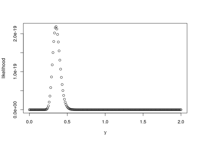
We can see a clear peak in the likelihood at around values of γ = 0.3 and γ = 0.4. Actually, the maximum can be easily found as
gamma[which.max(out)]
## [1] 0.3517588
Notice the y-scale in the plot. A value of 2e-19 denotes
2 × 10 − 19 = 0.0000000000000000002, a very small number! The
likelihood here is the product of 200 values between 0 and 1. Even if we
are able to predict the choices well, this will quickly become so small
that computers can’t represent it with sufficient precision. To avoid
such numerical problems, it is easier to work with the (natural)
logarithm of the likelihood. As an added bonus, the logarithm of a
product is the same as the sum of the logarithm of the elements in that
product: log (a × b) = log (a) + log (b), and sums can be easier
to work with. The following function computes the log-likelihood
l(γ|C1, …, C200, R1, …, R200) = log P(C1, …, C200|γ, R1, …, R200)
(note that here a small l refers to the log likelihood, while the
capital L used previously to the likelihood, i.e. l = log L)
kf_sm_logLik <- function(par,data) {
  gamma <- par[1]
  choice <- data$deck
  reward <- data$payoff
  m <- kalman_filter(choice,reward,4,0,1000,16,16)$m
  p <- softmax_choice_prob(m,gamma)
  lik <- p[cbind(1:nrow(data),choice)]
  logLik <- sum(log(lik))
  return(logLik)
}
A logarithm is a monotone transformation, meaning that the maximum of the logarithm of a function is at the same value as the maximum of the original function. Thus, while the plot of the log-likelihood looks quite different to the plot of the likelihood, we again can see that the maximum is around values of γ = 0.3 and γ = 0.4:
out <- rep(NA,length=length(gamma))
for(i in 1:length(gamma)) out[i] <- kf_sm_logLik(gamma[i],tdat)
plot(gamma,out,ylab="log-likelihood",xlab=expression(gamma))
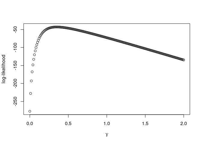
Indeed, we can see that the maximum is at the same value:
gamma[which.max(out)]
## [1] 0.3517588
While the grid was reasonably fine-grained, and the (log)-likelihood looks like a smooth and unimodal function, it is unlikely that the maximum found at γ̂ = 0.3517588 is the true maximum. If we had included more grid points around this value, another point may have been the maximum. We could choose to run the same procedure again with a new, finer grid surrounding the current maximum. This would get us ever closer to the true maximum. Effectively, this is what numerical optimization algorithms try to do “automatically”, exploring the function to get ever closer to the optimum until no there is no further improvement and the algorithm has converged. A small technicality is that numerical optimization routines tend to be formulated for function minimization rather than maximization. We thus need to reformulate the problem of finding the maximum of the log-likelihood function as one of finding the minimum of the negative log-likelihood function. The function to be optimized is then simply the likelihood multiplied by -1 (or any other negative value):
kf_sm_negLogLik <- function(par,data) {
  -kf_sm_lik(par,data)
}
Having defined the function to be optimized, we can now use R’s optim
function to find the maximum likelihood value of γ:
optim(par=.35,fn=kf_sm_negLogLik,data=tdat)
## Warning in optim(par = 0.35, fn = kf_sm_negLogLik, data = tdat): one-dimensional optimization by Nelder-Mead is unreliable:
## use "Brent" or optimize() directly

## $par
## [1] 0.35
##
## $value
## [1] -2.189173e-19
##
## $counts
## function gradient
##        2       NA
##
## $convergence
## [1] 0
##
## $message
## NULL
The first argument to optim is a starting value for the parameter, and
the second argument the function to be optimized. We also provide the
data argument which that function needs to evaluate the likelihood.
Even though we provided a good starting value based on our grid search,
the function doesn’t seem to have done it’s job, and returns as best
value under par the starting value. The reason for this is clear from
the warning message, which states that the default Nelder-Mead algorithm
is unreliable for unidimensional optimization, and suggests to use the
Brent algorithm instead:
optim(par=.35,fn=kf_sm_negLogLik,method="Brent",lower=0,upper=4,data=tdat)
## $par
## [1] 0.3501026
##
## $value
## [1] -2.189178e-19
##
## $counts
## function gradient
##       NA       NA
##
## $convergence
## [1] 0
##
## $message
## NULL
This algorithm searches with a specified range (here between 0 and 4), and finds the maximum at γ̂ = 0.3501026, which is close to the maximum found by grid search, but not identical, presumably because of the higher precision of this numerical optimization routine compared to grid search.
Assuming all parameters are unknown
Now that we know a little more about maximum likelihood estimation, let’s focus on estimating all the parameters of the Kalman filter with softmax model. In addition to γ, we will also attempt to estimate the parameters of the Kalman filter, which are the prior mean (μ0), prior variance (σ02), the innovation variance (σξ2), and noise variance (σϵ2). Letting θ = (γ, μ0, σ02, σξ2, σϵ2) denote the full set of parameters, the following function computes the negative log-likelihood \(\begin{align} - l(\theta|C_{1:200},R_{1:200}) &= - \log P(C_{1:200}|\theta,R_1,\ldots,R_{200})\\ &= - \log P(C_1|\theta,R_1) - \log P(C_2|\theta,R_1,C_1) - \ldots - \log P(C_{200}|\theta,C_{1:199},R_{1:199}) \\ &= - \sum_{t=1}^T \log P(C_t|\theta, C_{0:(t-1)}, R_{0:(t-1)})\end{align}\)
kf_sm_negLogLik <- function(par,data) {
  gamma <- par[1]
  mu0 <- par[2]
  sigma0_sq <- par[3]
  sigma_xi_sq <- par[4]
  sigma_epsilon_sq <- par[5]
  choice <- data$deck
  reward <- data$payoff
  m <- kalman_filter(choice,reward,4,mu0,sigma0_sq,sigma_xi_sq,sigma_epsilon_sq)$m
  p <- softmax_choice_prob(m,gamma)
  lik <- p[cbind(1:nrow(data),choice)]
  negLogLik <- -sum(log(lik))
  return(negLogLik)
}
Optimizing this function with the Nelder-Mead algorithm gives:
est <- optim(c(1,0,1000,16,16),kf_sm_negLogLik,data=tdat)
est$par
## [1] 3.307111e-01 -3.658455e+00 1.096434e+03 -1.140466e-02 -8.992243e-03
The estimate of γ is quite close to what we found previously. However, both the estimates of the innovation and noise variance are negative, which doesn’t make sense as a variance should be equal to or greater than 0…
Constraining and transforming parameters
When estimating parameters with numerical optimization, we should make
sure that the optimization algorithm “knows” about bounds and
constraints on the parameters (such as that variances
σ2 ≥ 0). In this case, we have lower bounds on some of the
parameters, which are a form of “box-constraints” which can be supplied
to optim:
est <- optim(par=c(1,0,1000,16,16),fn=kf_sm_negLogLik,lower=c(0,-Inf,0,0,0),data=tdat)
## Warning in optim(par = c(1, 0, 1000, 16, 16), fn = kf_sm_negLogLik, lower =
## c(0, : bounds can only be used with method L-BFGS-B (or Brent)
est
## $par
## [1]    0.332912   -3.746678 1000.002501   17.887978   14.016911
##
## $value
## [1] 41.59932
##
## $counts
## function gradient
##       27       27
##
## $convergence
## [1] 0
##
## $message
## [1] "CONVERGENCE: REL_REDUCTION_OF_F <= FACTR*EPSMCH"
First of all, note the warning; by supplying constraints, optim has
switched to the “L-BFGS-B” algorithm. Secondly, while the algorithm has
converged to a solution, the estimates of the variances are quite close
to the starting values. This is not necessarily cause for concern if we
have given good starting values (more on starting values later), but it
may point to issues in the model or estimation (more about this later as
well).
Another way to deal with bounds on the parameters is to reparameterize the model in such a way that the transformed parameters are boundless. We can then use unconstrained optimization, which may sometimes provide better estimates, although there are some caveats. For example, if we need a parameter which is strictly positive, i.e. θ > 0, we can use a log transform and optimize θ′ = log (θ) instead of θ itself. The logarithm of the lower bound 0 is log (0) = − ∞, while the logarithm of ∞ is log (∞) = ∞. Hence, if 0 < θ < ∞, then − ∞ < θ′ < ∞, so the to-be-optimized transformed parameter is unbounded. Some useful transformations for parameters with lower and/or upper bounds are listed in the table below. Once we have the optimal value for θ′, we can use the inverse transform to get the optimal value for the original parameter θ (e.g., θ = exp (θ′).
| Type | Formulation | Transformation | Inverse |
|---|---|---|---|
| Lower bound | θ > a | θ′ = log (θ − a) | θ = a + exp (θ′) |
| Upper bound | θ < b | θ′ = log (b − θ) | θ = b − exp (θ′) |
| Both | a < θ < b | $\theta' = \log \frac{(\theta-a)/(b-a)}{1 - (\theta-a)/(b-a)}$ | $\theta = a + \frac{b-a}{1 + \exp(-\theta')}$ |
Assuming that all the variance parameters are strictly positive, we can
use a simple log transformation for each (i.e., setting a = 0 in the
table above). The optim function can then again be used to optimize
the transformed parameters. Note that in the function to compute the
likelihood, we then first use the inverse transformation to turn the log
variances back into variances:
kf_sm_negLogLik_t <- function(par,data) {
  gamma <- par[1]
  mu0 <- par[2]
  # use inverse transform on variance parameters:
  sigma0_sq <- exp(par[3])
  sigma_xi_sq <- exp(par[4])
  sigma_epsilon_sq <- exp(par[5])
  choice <- data$deck
  reward <- data$payoff
  m <- kalman_filter(choice,reward,4,mu0,sigma0_sq,sigma_xi_sq,sigma_epsilon_sq)$m
  p <- softmax_choice_prob(m,gamma)
  lik <- p[cbind(1:nrow(data),choice)]
  negLogLik <- -sum(log(lik))
  return(negLogLik)
}
Running the optimization with this function gives:
est <- optim(c(1,0,log(1000),log(16),log(16)),kf_sm_negLogLik_t,data=tdat)
est
## $par
## [1]  0.333998 -3.571629 14.936633 -1.788288 -2.014682
##
## $value
## [1] 41.57891
##
## $counts
## function gradient
##      442       NA
##
## $convergence
## [1] 0
##
## $message
## NULL
Note that the value (the minimized negative log-likelihood) is quite close to that found with the L-BFGS-B algorithm. To compare the parameter estimates, we transform them back to the original parameters:
c(est$par[1:2],exp(est$par[3:5]))
## [1] 3.339980e-01 -3.571629e+00 3.068296e+06 1.672463e-01 1.333629e-01
This shows that while the likelihood is very similar, the parameter estimates are very different. In particular, the initial variance is much larger, while the innovation and error variance are much smaller. How can that be?
Local minima and starting values
One possibility is that there are local minima in the negative log-likelihood function. Numerical optimization routines are only guaranteed to return a local minimum. To see this in action, let’s define a function of two parameters with quite a few local minima:
loc_min <- function(x) {
  # x is a vector with 2 elements, x[1] and x[2]
  1e+5*(x[1]/20)*sin(x[1]/20)*(x[2]/20)*sin(x[2]/20)*dnorm(x[1],10,100)*dnorm(x[2],10,50)
}
The function is based on two sinusoid functions, and also uses two
normal densities so that there actually is a global minimum. Let’s plot
this function for a range of values of x[1] and x[2]:
tmp <- expand.grid(seq(-300,300,length=100),seq(-300,300,length=100))
tmp[,3] <- apply(tmp,1,loc_min)
loc_min_dat <- data.frame(x=tmp[,1],y=tmp[,2],z=tmp[,3])
library(ggplot2)
ggplot(loc_min_dat,aes(x=x,y=y,fill=z)) + geom_raster()
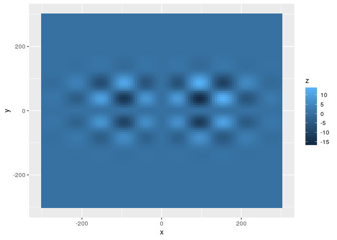
If we start the search in the middle of the plot, we get:
optim(c(0,0),loc_min)
## $par
## [1] 0 0
##
## $value
## [1] 0
##
## $counts
## function gradient
##        3       NA
##
## $convergence
## [1] 0
##
## $message
## NULL
Clearly, that didn’t work out very well. We started in a local minimum and the search did not go far enough beyond that to find out that there are better local minima. If, instead we start the search from a point in the upper-right quadrant, we get:
optim(c(50,50),loc_min)
## $par
## [1] 39.76354 86.89694
##
## $value
## [1] -6.877566
##
## $counts
## function gradient
##       91       NA
##
## $convergence
## [1] 0
##
## $message
## NULL
which is closer, but not quite the global maximum. A more “educated guess” for the starting values provides the correct answer:
optim(c(100,50),loc_min)
## $par
## [1] 95.05231 37.49262
##
## $value
## [1] -16.19015
##
## $counts
## function gradient
##       59       NA
##
## $convergence
## [1] 0
##
## $message
## NULL
In this case, as there were two parameters, it was straightforward to plot the objective function and find a reasonable starting values. When there are more than two parameters, this isn’t as easy. Generally, it is good practice to optimise from a wide range of starting values. For instance, we can create a grid of 2500 starting values and optimise from each cell in the grid as follows:
# define a set of starting values:
starting_values <- expand.grid(seq(-300,300,length=50),seq(-300,300,length=50))
# use apply to call optim for each starting value
opt <- apply(starting_values,1,function(x) optim(x,fn=loc_min))
# find the element in opt with the lowest value
opt[[which.min(unlist(lapply(opt,function(x) x$value)))]]
## $par
##     Var1     Var2
## 95.05337 37.49203
##
## $value
## [1] -16.19015
##
## $counts
## function gradient
##      115       NA
##
## $convergence
## [1] 0
##
## $message
## NULL
This repeated optimization for a large number of starting values was
feasible here because the evaluation of the loc_min function was
rather quick. For more involved computations, as is often the case with
calculating likelihoods, a smaller number of gridpoints will probably
have to be used. Also, when dealing with more parameters, the resolution
for each parameter may also have to be limited. Another option is to,
rather than optimise for each starting value, to simply compute the
likelihood for each starting value, and only perform the actual
optimization for the most promising starting value, or even better, for
a set of promising starting values. A middle way is to perform
optimization for a limited number of iterations for each starting value,
and then proceed with a (set of) promising starting value(s):
# set the maximum number of iterations for each initial optim run:
startIter <- 20
# set the number of values for which to run optim in full
fullIter <- 5
# define a set of starting values
starting_values <- expand.grid(seq(-300,300,length=50),seq(-300,300,length=50))
# call optim with startIter iterations for each starting value
opt <- apply(starting_values,1,function(x) optim(x,fn=loc_min,control=list(maxit=startIter)))
# define new starting values as the fullIter best values found thus far
starting_values_2 <- lapply(opt[order(unlist(lapply(opt,function(x) x$value)))[1:fullIter]],function(x) x$par)
# run optim in full for these new starting values
opt <- lapply(starting_values_2,optim,fn=loc_min)
# find the element in opt with the lowest value
opt[[which.min(unlist(lapply(opt,function(x) x$value)))]]
## $par
##     Var1     Var2
## 95.05348 37.49084
##
## $value
## [1] -16.19015
##
## $counts
## function gradient
##       53       NA
##
## $convergence
## [1] 0
##
## $message
## NULL
The more starting values you use, and the more optimization iterations
you use for each, the better. Instead of creating starting values on a
regular grid, you can also generate starting values randomly within the
region of parameter space you are interested in. A useful tool to create
a set of pseudo-random starting values which provides good coverage of
the region is to use a so-called Sobol sequence. The package randtools
provides a function to generate such sequences. It generates a set of
multivariate values which are between 0 and 1 on all dimensions. To make
these numbers fall within the region of interest (e.g., between -300 and
300), we can simply transform these. The function below does so:
library(randtoolbox)
## Loading required package: rngWELL

## This is randtoolbox. For an overview, type 'help("randtoolbox")'.
generate_starting_values <- function(n,min,max) {
  if(length(min) != length(max)) stop("min and max should have the same length")
  dim <- length(min)
  # generate Sobol values
  start <- sobol(n,dim=dim)
  # transform these to lie between min and max on each dimension
  for(i in 1:ncol(start)) {
    start[,i] <- min[i] + (max[i]-min[i])*start[,i]
  }
  return(start)
}
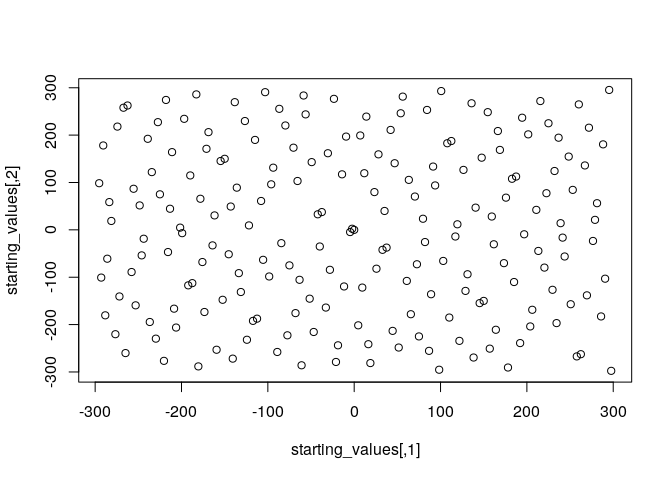
Generating starting values with this method and plotting them shows that they provide a reasonably even coverage of the whole parameter space:
set.seed(123)
starting_values <- generate_starting_values(200,min=rep(-300,2),max=rep(300,2))
plot(starting_values)
A final alternative worth mentioning is to use a stochastic optimization
routine. Most optimization methods implemented in the optim function
are deterministic, and when supplied with the same starting value, will
produce the same outcome. There is one exception to this, which is
simulated annealing, which can be called through optim(method="SANN").
This method will, from a given starting point, look randomly for new
candidate values by sampling these from a multivariate Normal
distribution centered on the current candidate. By slowly decreasing the
variance of this multivariate Normal (“decreasing the temperature”), the
method can successfully approach the global optimum. In principle, it is
guaranteed to arrive at the global optimum in the limit (with an
infinite number of iterations). In practice, the performance depends
crucially on aspects such as the cooling schedule (how quickly the
variance of the multivariate Normal decreases). Another stochastic
optimization routine that I have had good results from is differential
evolution optimization, implemented in the DEoptim package. The
DEoptim function in that package will search stochastically within a
specified region of parameter space to find the global minimum. Like the
SANN method in optim, the final result is a random variable. To
reproduce results exactly, you should thus fix the random seed (and it
may be worth running it a few times with different random seeds). The
following code runs this algorithm:
library(DEoptim)
set.seed(234)
opt <- DEoptim(loc_min,lower=c(-300,-300),upper=c(300,300),control=DEoptim.control(trace=FALSE))
The optimum value found is:
opt$optim$bestmem
##     par1     par2
## 95.05337 37.49203
which is very close to the earlier best results we found.
We can apply this routine to the problem of estimating the parameters of the Kalman filter + Softmax model. As this function searches within a specified range of parameter values, we do not need to transform parameters to make them unbounded. However, we do need to specify bounds for all parameters.
kf_sm_negLogLik_DE <- function(par,data) {
  negLL <- kf_sm_negLogLik(par,data)
  if(is.na(negLL)) negLL <- Inf
  return(negLL)
}
est_DE <- DEoptim(kf_sm_negLogLik_DE,lower=c(0,-100,0.00001,0.00001,.00001),upper=c(10,100,2000,100,100),data=tdat,control=DEoptim.control(trace=FALSE))
est_DE$optim$bestmem
##          par1          par2          par3          par4          par5
##    0.33404973   -3.57434675 1986.03849803    0.04278931    0.03404828
While the values of γ and μ0 are close to those found earlier, the variance parameters are again quite different.
Parameter identifiability
Although perhaps not immediately obvious from all the above, the Kalman filter + softmax model suffers from quite a “severe” problem: not all parameters are identifiable. Roughly, identifiability for a statistical model means that if we supply the model with different parameter values, the model should imply a different probability distribution over the data. This means that if p(Y|θ1) = p(Y|θ2) for almost all Y, this implies that θ1 = θ2. When each different setting of the model parameters implies a different probability distribution over the data, then in principle, given unlimited data, we should be able to identify the true parameters. For a limited dataset, identifiability implies that there is a unique global maximum of the likelihood value.
For the Kalman filter + softmax model, this is not the case. It turns out that we can multiply each of the variance parameters (v0, σξ2, and σϵ2) by a common scaling factor b and obtain exactly the same likelihood:
kf_sm_negLogLik(c(.3,0,1000,16,16),tdat)
## [1] 43.6253
kf_sm_negLogLik(c(.3,0,20*1000,20*16,20*16),tdat)
## [1] 43.6253
kf_sm_negLogLik(c(.3,0,.002*1000,.002*16,.002*16),tdat)
## [1] 43.6253
Some thinking shows why this is the case. Firstly, the softmax choice rule only cares about the (prior predictive) means mt, j of the options. Secondly, the Kalman filter updates for these means are defined (see also the previous blog post) as:
mt, j = mt − 1, j + kt, j(Rt − mt − 1, j).
with the Kalman gain
\[k_{t,j} = \begin{cases} \frac{v_{t-1,j} + \sigma_\xi^2}{v_{t-1,j} + \sigma_\xi^2 + \sigma_\epsilon^2} && \text{ if } C_t = j \\ 0 && \text{ otherwise } \end{cases}\]Multiplying each variance term by b > 0 for the first update at t = 1 gives exactly the same Kalman gain:
\[\frac{b v_{0,j} + b \sigma_\xi^2}{b v_{0,j} + b \sigma_\xi^2 + b \sigma_\epsilon^2} = \frac{v_{0,j} + \sigma_\xi^2}{v_{0,j} + \sigma_\xi^2 + \sigma_\epsilon^2}.\]It is also straightforward to show that the resulting posterior variance is always the value of the posterior variance with b = 1 multiplied by b. This means that for any update at any time t, the Kalman gain is the same for any value of b > 0. As a result, the posterior means are also the same, whatever the value of b!
This means that we cannot determine the true value of all three
parameters, σ02, σξ2,
and σϵ2. Effectively, we need to choose a
value for b by fixing one of these variances to a particular value. In
Speekenbrink and Konstantinidis (2015), we chose to fix
σ02 to an arbitrary value
(σ02 = 1000). As an alternative, we can choose
to fix the noise variance to the objective value
σϵ2 = 16. With this choice, we scale the
remaining variances with respect to the objective noise, which might
give more readily interpretable parameters. This is done in the
following variant of kf_sm_negLogLik_t, now called
kf_sm_negLogLik_t2:
kf_sm_negLogLik_t2 <- function(par,data) {
  gamma <- par[1]
  mu0 <- par[2]
  sigma0_sq <- exp(par[3])
  sigma_xi_sq <- exp(par[4])
  sigma_epsilon_sq <- 16
  choice <- data$deck
  reward <- data$payoff
  m <- kalman_filter(choice,reward,4,mu0,sigma0_sq,sigma_xi_sq,sigma_epsilon_sq)$m
  p <- softmax_choice_prob(m,gamma)
  lik <- p[cbind(1:nrow(data),choice)]
  negLogLik <- -sum(log(lik))
  if(is.na(negLogLik) | negLogLik == Inf) negLogLik <- 1e+300
  return(negLogLik)
}
As a check, we can see that we now can’t multiply the remaining variance parameters by a common factor b and obtain the same negative log likelihood:
kf_sm_negLogLik_t2(c(.3,0,log(1000),log(16)),tdat)
## [1] 43.6253
kf_sm_negLogLik_t2(c(.3,0,log(20*1000),log(20*16)),tdat)
## [1] 45.75205
kf_sm_negLogLik_t2(c(.3,0,log(.002*1000),log(.002*16)),tdat)
## [1] 100.5011
So, let’s see if we can apply what we have learned so far to estimate the remaining parameters:
starting_values <- generate_starting_values(200,min=c(.001,-100,log(.0001),log(.0001)),max=c(10,100,log(10000),log(100)))
opt <- apply(starting_values,1,function(x) optim(x,fn=kf_sm_negLogLik_t2,data=tdat,control=list(maxit=startIter)))
starting_values_2 <- lapply(opt[order(unlist(lapply(opt,function(x) x$value)))[1:5]],function(x) x$par)
opt <- lapply(starting_values_2,optim,fn=kf_sm_negLogLik_t2,data=tdat)
bestopt <- opt[[which.min(unlist(lapply(opt,function(x) x$value)))]]
bestopt
## $par
## [1]  0.3340826 -3.5692984 16.2083402  2.9991466
##
## $value
## [1] 41.57892
##
## $counts
## function gradient
##      471       NA
##
## $convergence
## [1] 0
##
## $message
## NULL
c(bestopt$par[1:2],exp(bestopt$par[3:4]))
## [1] 3.340826e-01 -3.569298e+00 1.094442e+07 2.006840e+01
These are reasonable estimates. Note that the initial uncertainty (σ02) is very large. This is not necessarily unreasonable; it simply implies high initial Kalman gains (i.e. “learning rates”).
Estimating the Kalman filter and UCB
As we learned that the Kalman filter and softmax model is not completely identifiable, we should keep this in mind when trying to estimate the other models, such as the Kalman filter and UCB model. But first we need to tackle another issue for this particular model: as defined in the last blog post, the UCB rule is deterministic. Fitting deterministic models by maximum likelihood tends to give problems, especially when dealing with data from human participants. It may be unlikely that a human follows the UCB rule exactly, even if it provides a good (but not perfect) description of their behaviour. In other words, we would like to allow for some (stochastic) deviations from this rule. There are different ways in which to turn a deterministic rule into a probabilistic one. One idea is to implement a “trembling hand”, such that with a particular probability 1 − ϵ, the person deviates from the UCB rule. We would then need to define what happens in that case. A simple option is to state that the person then chooses uniformly between the other options. But that may be unlikely. Would it not be more reasonable to expect that, if a person deviates, the probability of choosing an option which looks better should be higher than an option that looks worse? If so, then another option is to use a softmax function over the main ingredient of the UCB rule, namely the upper confidence bound. So similar to the softmax function we have dealt with so extensively, we can define a probabilistic version of the UCB rule as
\[P(C_{t} = j|\theta,C_{0:(t-1)},R_{0:(t-1)}) = \frac{\exp \gamma (m_{t-1,j} + \beta \sqrt{v_{t-1,j} + \sigma^2_\xi})}{\sum_{k=1}^4 \exp \gamma (m_{t-1,k} + \beta \sqrt{v_{t-1,k} + \sigma^2_\xi})}\]Is this model identifiable? We know from the previous discussion that if we multiply all variances by a common scaling factor, we obtain exactly the same values for mt, j. However, we would get other values for the $\beta \sqrt{v_{t-1,j} + \sigma^2\xi}$ term, which would become $\beta \sqrt{b v{t-1,j} + b \sigma^2_\xi}$. Let’s consider b = 2. As β is a free parameter, this could account for this increased prior predictive variance by reducing its value to $\beta/\sqrt{b}$, which would then again give exactly the same predictions. So, again not all parameters are identifiable, just as for the softmax rule. To resolve the unidentifiability issue, we can again fix one of the variance parameters to a particular value, such as σϵ = 16.
ucb_choice_prob <- function(m,ppsd,gamma,beta) {
  prob <- exp(gamma*(m + beta*ppsd))
  prob <- prob/rowSums(prob)
  return(prob)
}

kf_ucb_negLogLik_t2 <- function(par,data) {
  gamma <- exp(par[1])
  beta <- exp(par[2])
  mu0 <- par[3]
  sigma0_sq <- exp(par[4])
  sigma_xi_sq <- exp(par[5])
  sigma_epsilon_sq <- 16
  choice <- data$deck
  reward <- data$payoff
  kf <- kalman_filter(choice,reward,4,mu0,sigma0_sq,sigma_xi_sq,sigma_epsilon_sq)
  m <- kf$m
  ppsd <- sqrt(kf$v + sigma_xi_sq)
  p <- ucb_choice_prob(m,ppsd,gamma,beta)
  lik <- p[cbind(1:nrow(data),choice)]
  negLogLik <- -sum(log(lik))
  if(is.na(negLogLik) | negLogLik == Inf) negLogLik <- 1e+300
  return(negLogLik)
}
Using a similar procedure to estimate the parameters as before gives:
starting_values <- generate_starting_values(600,min=c(log(.001),log(.001),-10,log(.0001),log(.0001)),max=c(log(10),log(10),10,log(10000),log(100)))
opt <- apply(starting_values,1,function(x) optim(x,fn=kf_ucb_negLogLik_t2,data=tdat,control=list(maxit=startIter)))
starting_values_2 <- lapply(opt[order(unlist(lapply(opt,function(x) x$value)))[1:5]],function(x) x$par)
opt <- lapply(starting_values_2,optim,fn=kf_ucb_negLogLik_t2,data=tdat)
bestopt <- opt[[which.min(unlist(lapply(opt,function(x) x$value)))]]
bestopt
## $par
## [1]  -1.096660 -19.275952  -3.572989  18.411301   2.999183
##
## $value
## [1] 41.57891
##
## $counts
## function gradient
##      272       NA
##
## $convergence
## [1] 0
##
## $message
## NULL
c(exp(bestopt$par[1:2]),bestopt$par[3],exp(bestopt$par[4:5]))
## [1] 3.339848e-01 4.251680e-09 -3.572989e+00 9.906640e+07 2.006914e+01
Interestingly, the values of γ, μ0, σ02 and σξ2 are quite close to those found for the Kalman filter + softmax model. This may be because the value of β is quite close to 0, and when β = 0, the Kalman filter + UCB model is identical to the Kalman filter + softmax model.
Conclusion
As this post is already very long, we will save the estimating the Kalman filter + Thompson sampling model for the next post in this series. To conclude for now, we have covered a number of important topics. We have introduced maximum likelihood estimation, and covered how to numerically optimize the likelihood function to obtain maximum likelihood estimates in practice. We have looked at different ways to deal with simple constraints on the parameters, and have illustrated the fact that numerical optimization routines are only guaranteed to return a local optimum. To increase the chances of finding the global optimum, it is useful to try a good range of starting values. We then stumbled upon a very important topic in modelling, which is unfortunately often overlooked: parameter identifiability. Roughly, if model parameters are identifiable, this means that a different choice of parameters should result in a different value of the log likelihood. If a model is not identifiable, as is the case for the Kalman filter with softmax and UCB, then the parameter values returned by an optimization routine are meaningless. Fixing the value of a particular parameter to an a priori value in this case resolved the unidentifiability problem.
References
Speekenbrink, M., and E. Konstantinidis. 2015. “Uncertainty and Exploration in a Restless Bandit Problem.” Topics in Cognitive Science 7 (2): 351–67. https://doi.org/10.1111/tops.12145.
Comments