Modeling reinforcement learning (Part I): Defining and simulating RL models

This post is the first in a series on fitting reinforcement learning (RL) models to describe human learning and decision making. Using example data from Speekenbrink and Konstantinidis (2015), we will go through the various steps involved, inluding the definition of a model, estimating its parameters, and doing inference and model comparison. Many students and researchers are interested in using computational models to describe human cognition, but don’t know where to start. I hope that this series will offer a useful introduction to computational modelling of human cognition.

In any modelling exercise, it is crucial to have a good understanding of the models. How do they work? What role do the parameters play? Therefore, in this first post, I will:

• introduce the restless bandit task
• describe three (Bayesian) reinforcement learning algorithms, all based on the Kalman filter with different choice rules (softmax, UCB, and Thompson sampling)
• show how to implement an RL agent in R
• simulate the choices of the different RL agents and assess how performance depends on key parameters.

Restless bandits

Imagine you just moved to a new city for work. There are different options to get from your new home to work: walking, cycling, car, taxi, bus, and the tube (metro). Initially, you don’t know how long each option takes, or how much it costs. You want to spend as little time and money as possible on your commute. By trying each option, you can learn about the temporal and financial costs. On each day, these may vary. For instance, if traffic is busy, a journey by taxi will take longer and cost more than when traffic is quiet. Traffic conditions will fluctuate from day to day, but there may also be longer lasting changes. For instance, major road works may make traffic busier on unaffected routes for a prolonged period . Crucially, you will only learn about the temporal and financial costs of a particular mode of transport on a particular day by choosing to travel that way. If you take the tube, you don’t know how long the journey would have taken if you had cycled. This is an example of a restless multi-armed bandit task: you need to repeatedly choose between different alternatives which have costs and rewards that vary randomly from moment to moment but which may also be subject to longer lasting changes (due to e.g. price changes and road works), and your goal is to accumulate as much reward (or incur the least amount of loss) as possible over all choices.

A multi-armed bandit task involves repeatedly choosing between alternatives that offer stochastic rewards, with the primary goal to accumulate as much reward as possible. Iniitially, little or nothing is known about each option’s expected reward, but by trying options and observing the rewards they offer, an agent can learn about the options and use this knowledge to make better choices. As rewards can only be obtained (and observed) by choosing an option, good performance in this tasks requires balancing exploitation (choosing options which the agent believes are good) and exploration (choosing options about which relatively little is known, in order to learn more about them). The term multi-armed bandit refers to a gambling setting. A one-armed bandit is another name for a slot machine. The notion of a multi-armed bandit involves a more complicated slot machine with multiple arms, each with a different unknown probability of winning. Compared to a collection of one-armed bandits, the multi-armed bandit, being a single system, allows for dependencies between the arms, such as that pulling one arm might change the reward distribution of another arm. Here, we do not consider such dependencies, so rather than talking of different arms of a single bandit, I may refer to the arms as different bandits.

Optimally solving the exploration-exploitation dilemma is difficult and often impossible. It requires determining the likely consequences of an immediate action on future actions and their rewards. This is only tractable in specific cases (Gittins, Glazebrook, and Weber 2011), and a restless bandit is not one of those. Generally, workable RL algorithms rely on heuristics rather than optimal strategies. In particular, they tend to be “greedy” in the sense that only the immediate consequences of an action are considered. They do not directly tackle the problem of determining how information gained from trying an action will be used in later decisions.

In the study reported in Speekenbrink and Konstantinidis (2015), participants made choices for 200 trials. Each option gave a continuous reward drawn from a Normal distribution with a constant variance but time-varying mean. Let R_t, j be the stochastic reward option j provides at time t. The following two equations define our restless bandit:

In words, the reward R_t, j of option j at time t is equal to the sum of the mean reward (μ_t, j) and an error term (ϵ_t, j) drawn from a Normal distribution with mean of 0 and a variance equal to σ_ϵ². This is equivalent to the reward being drawn from a Normal distribution with mean μ_t, j and variance σ_ϵ². The means μ_t, j vary over time according to a random walk, such that the mean on time t is equal to the mean at time t − 1 and a disturbance term ξ_t, j which is drawn from a Normal distribution with mean 0 and variance σ_ξ². This is equivalent to the mean at time t being drawn from a Normal distribution with mean μ_{t − 1, j} and variance σ_ξ². We will refer to σ_ϵ² as the noise variance, and σ_ξ² as the innovation variance. The model presented above is a very simple example of a linear dynamical system or state-space model, and called the local-level model by Durbin and Koopman (2012).

The equations may be a little abstract, so let’s use R to simulate one instantiation of our restless bandit. We will follow Speekenbrink and Konstantinidis (2015), and set the noise variance to σ_ϵ² = 16, the innovation variance to σ_ξ² = 16, and initialize the means at μ₁ = ( − 60, −20, 20, 60). We will create one data frame mu to hold the time-varying means, and another data frame rewards to hold the stochastic rewards. The latter will be useful when we simulate the RL agents. To be able to replicate what I’m doing, we also initialize the random seed to a particular value, using set.seed(). Choosing a different value will give different results, and it can be insightful to try this.

set.seed(3) # set the random seed to replicate these results exactly
mu <- matrix(0.0,nrow=200,ncol=4) # to store the time-varying means
mu[1,] <- c(-60, -20, 20, 60) # initialize the means for t=1
for(t in 2:200) {
  mu[t,] <- mu[t-1,] + rnorm(4,mean=0,sd=4) # compute mean at t based on mean at t-1
}
rewards <- mu + rnorm(length(mu),mean=0,sd=4) # generate the stochastic rewards
mu <- as.data.frame(cbind(1:200,mu))
rewards <- as.data.frame(cbind(1:200,rewards))
colnames(rewards) <- colnames(mu) <- c("trial",paste0("A",1:4))

Plotting the means shows how restless our bandit really is, with option 4 being the best (in terms of average reward) for the first half of the task, while option 1 and 2 are better later on.

library(dplyr)
library(tidyr)
library(ggplot2)
mu %>%
  gather(key=option,value=mu,-trial) %>%
    ggplot(aes(x=trial,y=mu,colour=option)) + geom_line()

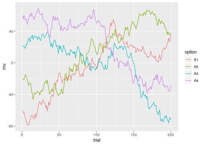
If an agent only explores initially, she might determine that option 4 is best, and then exploit this knowledge thereafter. But when only choosing option 4, she foregoes the chance to detect that after some time, other options become better. In restless bandits, it is wise to keep exploring occasionally!

Reinforcement learning models

We need a model to learn the mean rewards associated to each bandit, and a choice rule which uses this knowledge to make wise choices. For the learning part, we will use a Kalman filter. In this context, the Kalman filter can be viewed as a variant of the “delta-rule”, but with a time-varying learning rate that is adjusted according to uncertainty and the sources of variability in the environment. This provides a principled way to determine the appropriate learning rate, which can be difficult for the delta-rule. An additional advantage of the Kalman filter is that it provides posterior distributions for the mean reward of each option. These distributions do not only tell us what reward can be expected (i.e. the mean of this distribution is the expected reward), but also provide a measure of the uncertainty associated with those expectations (i.e., the variance of this distribution is a measure of the uncertainty of our expectations). We will combine the Kalman filter learning component with three choice rules, which determine which bandit to choose given the current estimates for all bandits. These choice rules are: (a) the “softmax” rule, which doesn’t take uncertainty into account, (b) the “upper confidence bound” rule, which promotes exploration for uncertain options through an exploration bonus, and (c) “Thompson sampling”, which also promotes exploration of uncertain options, but through a stochastic sampling mechanism.

Kalman filter

The Kalman filter (Kalman 1960; Kalman and Bucy 1961) is an optimal learning model for our restless bandits with Normally distributed rewards and time-varying means. The rewards can be viewed as noisy observations of the true underlying state of the bandit (the mean reward). In a way, the learning problem is similar to tracking a moving target from noisy measurements, a problem for which the Kalman filter was originally designed.

For each bandit j, the Kalman filter computes the mean m_t, j and variance v_t, j of the posterior distribution of the true average reward μ_t, j at time t. Assuming the prior distribution (before observing any rewards) is a Normal distribution: p(μ_0, j)=𝒩(m_0, j, v_0, j), these posterior distributions are also Normal distributions: p(μ_t, j ∣ 𝒟_t)=𝒩(m_t, j, v_t, j), where 𝒟_t = (R₁, C₁, …, R_t, C_t) denotes all the relevant information up to time t (the obtained rewards R_t and the identity of the bandit which led to this reward, provided by the choice variable C_t indicating which bandit was chosen at time t). Such a posterior distribution at time t provides a prior distribution for time t + 1, with one important change. Due to the random walk underlying the means, even if it were possible to completely accurately determine the mean at time t (in which case m_t, j = μ_t, j and v_t, j = 0), there would again be uncertainty about the mean at time t + 1. As the mean μ_{t + 1, j} is Normally distributed around μ_t, j, with variance σ_ξ², our prior distribution for the mean at time t + 1 would be 𝒩(m_t, j, σ_ξ²). Thus, a time-varying mean adds uncertainty. It is generally not possible to completely accurately determine the mean at time t, and the posterior uncertainty at time t, given by v_t, j, will feed into the prior uncertainty at time t + 1. This prior uncertainty is then equal to v_t, j + σ_ξ². Hence, the prior distribution at time t + 1 is: p(μ_{t + 1, j} ∣ 𝒟_t)=𝒩(m_t, j, v_t, j + σ_ξ²).

The Kalman filter provides an efficient way to calculate the parameters of these distributions sequentially. The mean of the posterior reward distribution at time t is computed as: m_t, j = m_{t − 1, j} + k_t, j(R_t − m_{t − 1, j}). This can be viewed as a variant of the delta-rule, which updates expectations m_t, j according to a reward prediction error RPE = R_t − m_{t − 1, j}. If the reward is higher than the expectation, the expectation is increased. If the reward is lower than the expectation, the expectation is decreased. The size of these updates is determined by the “learning rate” or Kalman gain k_t, j ∈ [0, 1]. The standard version of the “delta-rule” can be stated as: m_t, j = m_{t − 1, j} + α(R_t − m_{t − 1, j}), where α ∈ [0, 1] is a fixed learning rate. Thus, in the delta-rule, the learning rate is a constant, and invariant over time. In the Kalman filter, the learning rate or Kalman gain changes over time. In our bandit setting, the Kalman gain can be computed as:

Note that we make the Kalman gain dependent on whether an option was chosen or not. Recall that the variable C_t denotes the chosen bandit at time t. In a bandit setting, you only obtain information about the chosen option. If an option has not been chosen, there is no way to determine the relevant reward prediction error, and hence no basis to adjust the expected reward m_t, j. Because in our restless bandit, the means are equally likely to go up as down from one timepoint to the next (they are symmetrically distributed around the mean at the previous timepoint), it makes sense to keep the expected rewards the same if you have no new information. But because we know the mean reward will change over time, the uncertainty about the mean reward should increase when you receive no new information. This increase in uncertainty for unchosen options becomes clear when we look at the calculation of the posterior variance: v_t, j = (1 − k_t, j)(v_{t − 1, j} + σ_ξ²). This shows that the posterior variance v_j, t is a function of the prior variance v_{t − 1, j} + σ_ξ² (recall what was said earlier about the relation between posterior and prior distributions). For unchosen options, we have defined k_t, j = 0, so 1 − k_t, j = 1 and the posterior variance at time t + 1 is simply the sum of the posterior variance at time t and the innovation variance σ_ξ². For the chosen option, 1 − k_t, j lies between 0 and 1, and hence the posterior variance is smaller than the prior variance v_{t − 1, j} + σ_ξ². In short: observing a reward reduces uncertainty about the mean reward.

Let’s look a little more closely at the Kalman gain. It depends solely on three factors: the initial uncertainty (v_0, t), the error variance (σ_ϵ²), and the innovation variance (σ_ξ²). Let’s plot the value of the Kalman gain over time for different choices of these parameters:

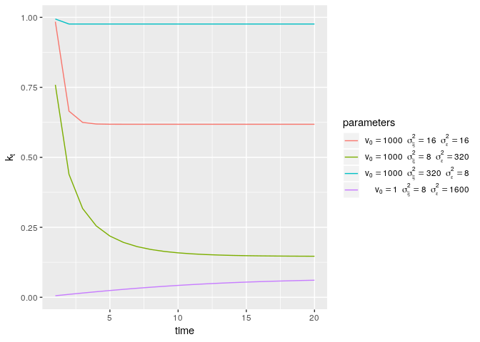
This plot shows that the Kalman gain generally decreases over time, but can also increase if the prior uncertainty (v₀) is very low. Also, the Kalman gain is higher when the innovation variance (σ_ξ²) increases relative to the noise variance (σ_ϵ²). Finally, the Kalman gain tends to converge quickly to a constant value, k_*, which is called the steady-state gain (Durbin and Koopman 2012):

Given this quick convergence to a constant learning rate, you might wonder why we bother with the Kalman filter over the simpler delta-rule, which has a constant learning rate from the outset. Well, as already mentioned, the Kalman filter allows you to determine the optimal learning rate, and provides not only point estimates of mean reward, but also a measure of the uncertainty in these estimates. Furthermore, and rather importantly for the bandit setting, the Kalman gain values plotted above are valid when the reward for a particular bandit is observed at each timepoint. In a bandit task, this is generally not the case, as choosing one option means that we don’t observe the reward of the remaining options. For unchosen options, the uncertainty increases, and with that the Kalman gain. So, in a bandit task, the Kalman filter allows the learning rate to depend on how often a bandit is chosen. If a bandit has not been chosen for some time, the Kalman filter allows you to quickly “get up to speed” when the bandit is chosen eventually. To see how this works, let’s pick one of the examples from the plot above, but assume the option is chosen (and hence the reward observed) only at timepoints 1, 2, 3, 10, 11, 15 and 16:

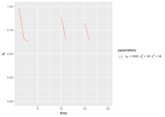
As this plot shows, the Kalman gain decreases whilst choosing an option, but increases again when an option has not been chosen for some time.

In summary, the Kalman filter provides a means to estimate expected rewards and the associated estimation uncertainty. We will now look at three different strategies to use this information and determine, at each timepoint, which bandit to choose.

Softmax choice

We will start with a rather simple choice rule, the so-called softmax rule (Sutton and Barto 1998). As the name suggests, this is a form of “soft” maximisation, meaning that the option with the highest expectation is chosen most of the time, but sometimes also options with lower expectations are chosen. In contrast to another choice rule, called epsilon-greedy (Sutton and Barto 1998), which usually chooses the option with the highest expectation, but otherwise chooses between the remaining options completely randomly, the softmax rule is a little cleverer, and can discount options for which the expectation is much lower than for other options. According to the softmax rule, the probability of choosing option j at time t is:

This can be viewed as first transforming each expectation by multiplying it with a common factor γ, and then taking the (natural) exponent. The last step makes sure that the resulting value is always positive. The γ parameter (sometimes also called the “inverse temperature”) scales the values: large values of γ increase the differences between options, low values decrease them. After this transformation, the rule can be viewed as determining the “relative goodness” of each option as the ratio of the transformed expectation over the sum of all transformed expectations.

Upper confidence bound (UCB) choice

The softmax choice rule is based purely on expected rewards, and doesn’t take the estimation uncertainty into account. Intuitively, if the estimation uncertainty is large, a lot can be learned by trying the bandit and observing its reward. In other words, high estimation uncertainty indicates a high potential benefit of exploring a bandit. But this is not all there is to exploration. Imagine there are two bandits, one with an expected reward of m_t, 1 = 0, and one with an expected reward of m_t, 2 = 1000. Let’s also assume that the estimation uncertainties are v_t, 1 = 1000 and v_t, 2 = 1. Now, there is much more uncertainty about option 1 than 2, which could indicate that exploring option 1 is beneficial. However, it is extremely unlikely that option 1 is actually better than option 2. As the posterior distribution of average reward is Normal, we can determine that with 99.99% confidence, the mean reward of option 1 lies between -123.031 and 123.031. So while exploring option 1 will reduce the estimation uncertainty, this increase in knowledge about option 1 is not likely to help us make better choices, as we can already be rather certain that option 2 is the best. As this example illustrates, exploration should be based on uncertainty and expected reward. The upper-confidence bound (UCB) strategy is a popular way to do this. It is based on the idea of computing confidence intervals around the expected rewards in order to determine whether it is worth exploring options.

For our Kalman filter model, prior distributions of mean reward at time t are Normal distributions, with mean m_{t − 1, j} and variance v_{t − 1, j} + σ_ξ². We can then state the UCB rule as follows:

In words, we choose an option j when \(m_{t-1,j} + \beta (\sqrt{v_{t-1,j} + \sigma^2_\xi})\) is larger than that same term for all options k that are not equal to option j. For a Normally distributed variable with mean m and standard deviation s, m + β**s is the upper limit of a confidence interval. Here, we have a Normally distributed variable with mean m_{t − 1, j} and standard deviation \(\sqrt{v_{t-1,j} + \sigma^2_\xi}\). Thus, for example, \(m_{t-1,j} + 1.96 \sqrt{v_{t-1,k} + \sigma^2_\xi}\) is the upper limit of the 95% confidence interval for the mean reward of option j. Choosing β ≈ 2.5758 would give us the upper limit of the 99% confidence interval. In words, the UCB rule is simply: choose the option with the highest upper confidence bound. Unlike the softmax rule, this is a deterministic strategy (although we might randomize the choice in the case where there are ties; more about that later).

One interpretation of the UCB rule is as a form of “optimism in the face of uncertainty”, inflating the expectations of each option by an amount that depends on uncertainty. So, each option is given an “uncertainty bonus”, and after this, we simply choose the option which looks the best as a result.

Thompson sampling

The last choice strategy we will look at is known as Thompson sampling (Thompson 1933). Like the UCB rule, it takes both expected rewards and estimation uncertainty into account. However, unlike the UCB rule, it is a stochastic strategy, and chooses options according to the probability that they have the highest mean reward. At timepoint t, we have, for each option, a prior distribution of the mean reward: p(μ_t, j ∣ 𝒟_t − 1)=𝒩(m_{t − 1, j}, v_{t − 1, j} + σ_ξ²). Using these prior distributions, we can derive, for each option, the (prior) probability that it has the highest mean, P(∀k ≠ j : μ_t, j > μ_t, k ∣ 𝒟_t − 1). While we could opt to always choose the option for which this probability is highest, this wouldn’t lead to exploration. Instead, we can opt to choose options randomly, with the probability of choosing an option equal to the prior probability that it has the highest mean reward. This is what Thompson sampling does. The Thompson sampling strategy can be stated formally as: P(C_t = j)=P(∀k ≠ j : μ_t, j > μ_t, k ∣ 𝒟_t − 1)

Thompson sampling is a form of Bayesian probablity matching. While probability matching is often considered dumb and/or irrational, this negative evaluation is really only true for single-shot decisions. In a bandit setting, probability matching in this way actually turns out to be a rather smart strategy, as it offers a principled way to balance exploration and exploitation.

For our case, where all relevant distributions are Normal, the probability that each option has the highest mean can be worked out analytically. I will show how in a future post. If we are just interested in making choices according to these probabilities, there is a simple way to do so without working them out. We can simply sample, for each option, a predicted mean reward from the prior distribution, and choose the option for which this sampled value is largest. This leads to the following alternative way to specify the Thompson sampling rule:

where \(\tilde{m}_{t,j}\) denotes a sample from the prior distribution of the mean rewards.

One advantage of Thompson sampling over the other two strategies is that it does not have any parameters which need to be set (such as γ for the softmax, and β for the UCB rule). Thompson sampling works solely on the prior predictive distributions.

Simulating RL agents

We now have a learning rule (the Kalman filter) and three choice rules (softmax, UCB, and Thompson sampling). We have described these mathematically, and worked out some details. But a lot of knowledge about the resulting RL strategies can be learned by simulating RL agents, and see how they behave in our restless bandit task. So let’s get to work.

Softmax

We will start by simulating an RL agent with a Kalman filter learning rule and the softmax choice rule. Below, I define a function rl_softmax_sim, which takes a matrix of all the rewards for all options, and the relevant parameters for the Kalman filter (m_0, j, v_0, j, σ_ξ², σ_ϵ²) and softmax rule (γ). In the main loop of the function, a choice is made according to the softmax rule, and then the resulting reward is collected, after which the Kalman filter is used to compute the parameters (m_t, j and v_t, j) of the posterior distributions of the mean reward.

rl_softmax_sim <- function(rewards,m0,v0,sigma_xi_sq,sigma_epsilon_sq,gamma) {
  nt <- nrow(rewards) # number of time points
  no <- ncol(rewards) # number of options
  m <- matrix(m0,ncol=no,nrow=nt+1) # to hold the posterior means
  v <- matrix(v0,ncol=no,nrow=nt+1) # to hold the posterior variances
  choice <- rep(0,nt) # to hold the choices of the RL agent
  reward <- rep(0.0,nt) # to hold the obtained rewards by the RL agent
  # loop over all timepoints
  for(t in 1:nt) {
    # use the prior means and compute the probability of choosing each option
    p <- exp(gamma*m[t,])
    p <- p/sum(p)
    # choose an option according to these probabilities
    choice[t] <- sample(1:4,size=1,prob=p)
    # get the reward of the choice
    reward[t] <- rewards[t,choice[t]]
    # set the Kalman gain for unchosen options
    kt <- rep(0,4)
    # set the Kalman gain for the chosen option
    kt[choice[t]] <- (v[t,choice[t]] + sigma_xi_sq)/(v[t,choice[t]] + sigma_xi_sq + sigma_epsilon_sq)
    # compute the posterior means
    m[t+1,] <- m[t,] + kt*(reward[t] - m[t,])
    # compute the posterior variances
    v[t+1,] <- (1-kt)*(v[t,] + sigma_xi_sq)
  }
  # return everything of interest
  return(list(m=m,v=v,choice=choice,reward=reward))
}

With this function, we can simulate RL agents with different settings of the parameters, and different rewards. In the first simulation, and all others later, we will use the following parameters for the Kalman filter: m_0, j = 0, v_0, j = 1000, σ_ξ² = 16, σ_ϵ² = 16. The prior mean and variance are reasonable for this task, and the innovation variance and and error variance are set to their true values. For this first simulation, we will additionally set γ = 1:

rewards_mat <- as.matrix(rewards[,-1]) # extract rewards from the rewards data.frame
set.seed(123) # set seed to replicate results exactly
# run the RL agent with
sim_softmax_100 <- rl_softmax_sim(rewards_mat,m0=0.0,v0=1000,sigma_xi_sq=16,sigma_epsilon_sq=16,gamma=1)

Let’s see how this agent performs in terms of the accumulated total reward, and also look at the options chosen:

sum(sim_softmax_100$reward)

## [1] 6281

table(sim_softmax_100$choice)

##
##   2   3
## 116  84

We can see that the agent never explored option 1 and 4, and accumulated a total reward of 6281.314. We don’t know whether this is any good. The maximum reward that the agent could have obtained (with exactly these randomly drawn rewards) is 10001.405, but this is not really a fair standard. We can also work out the expected reward if the agent always chose the option with the highest true mean reward, which is 10032.601. Comparing obtained rewards to the highest possible expected reward (i.e. the expected reward obtained by always choosing the option with the highest expected reward) is a common measure of the “regret” associated with following a particular RL strategy. In this case, the regret is 3751.287. We can also compare the performance of our RL agent to a “completely random agent”” who, at each time t, chooses uniformly between the options:

set.seed(123)
sum(rewards[cbind(1:200,sample(1:4,size=200,replace = TRUE))])

## [1] 5169

The agent performs somewhat better than random, but the difference is not that large.

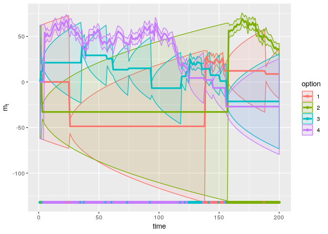
To get some more insight into the behaviour of our RL agent, let’s create a plot to show the choices of the agent, and the inferred mean rewards and 95% confidence bounds. This plot will be useful to inspect other RL agents as well, so I have created a function that can be used later on as well. In this function, I first create a data.frame with all the relevant information about choices, inferred means, and upper and lower bounds of the 95% confidence intervals for each option. I then use ggplot2 to plot the choices as dots at the bottom of the plot, the posterior means as lines, and the confidence bounds as ribbons around these lines:

plot_sim <- function(sim) {
  data.frame(trial=1:200,option=factor(rep(1:4,each=200)),m=as.numeric(sim$m[-201,]),mmax=as.numeric(sim$m[-201,]) + 1.96*sqrt(as.numeric(sim$v[-201,])),mmin=as.numeric(sim$m[-201,]) - 1.96*sqrt(as.numeric(sim$v[-201,]))) %>%
    ggplot(aes(x=trial,y=m,colour=option,fill=option)) + geom_ribbon(aes(ymin=mmin,ymax=mmax),alpha=.1) +
  geom_line(size=1.2) + geom_point(aes(x=trial,y=min(sim$m - 1.96*sqrt(sim$v)),colour=choice,fill=choice),data=data.frame(trial=1:200,choice=factor(sim$choice))) + xlab("time") + ylab(expression(m[t]))
}
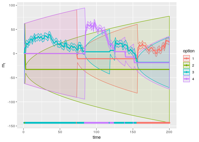
plot_sim(sim_softmax_100)

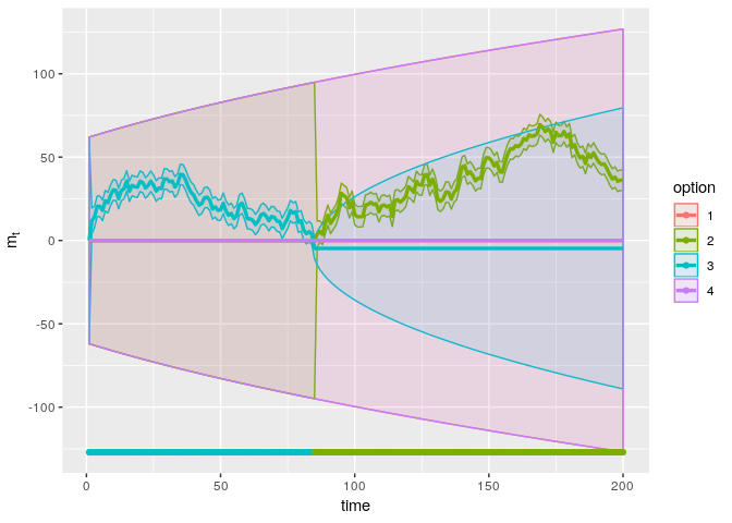
The resulting plot looks, I must admit, a little messy for this simulation. The dots at the bottom show that the agent chooses option 3 for some time, and then switches to option 2. The main panel shows the inferred mean reward of each option (solid line) and the 95% confidence interval around these estimates. During the initial period in which only option 3 is chosen, we can see that the uncertainty about the mean reward of this option is relatively small. Because the agent has not gained any information about the other options, the inferred mean reward of these options remains at the initial value (m_0, j = 0), while the uncertainty increases gradually. The posterior distributions are exactly the same for option 1, 2, and 4 during this time, and hence these are plotted on top of each other, making it difficult to discriminate between the options. After some time, the inferred mean reward of option 3 decreases to a value below 0. After that, all other options are deemed as more rewarding. The agent tries option 2, and finding that the reward is larger than 0, now infers that this option is better than option 1, 3, and 4. Because the inferred mean never decreases sufficiently, the agent keeps choosing option 2 from then on. As option 3 is no longer chosen, we can see the uncertainty about this option slowly increasing.

It looks as if the agent simply always chose the option with the highest inferred mean reward, only randomizing choice in the case of ties. This is like an agent who never explores, only exploits. To promote exploration, we may need to set the exploration parameter γ to a lower value, for instance to γ = .2:

set.seed(123)
sim_softmax_020 <- rl_softmax_sim(rewards_mat,m0=0.0,v0=1000,sigma_xi_sq=16,sigma_epsilon_sq=16,gamma=.2)
plot_sim(sim_softmax_020)

This plot looks a little more interesting. This softmax agent explores all options, although not so much initially. Generally, exploration is initiated when the average of the currently favoured option decreases sufficiently to be close to the estimated reward of other options. While decreasing γ has made the agent explore all options, the accumulated reward is actually lower than before, at 4374.505, meaning the regret is now 5658.097.

As these two examples show, the choice of γ is crucial in arriving at a good balance between exploration and exploitation. Below, we will try a range of γ values and check the resulting accumulated rewards:

gamma <- seq(0,3,length=100)
out <- rep(0,100)
for(i in 1:length(gamma)) {
  set.seed(123)
  sim <- rl_softmax_sim(rewards_mat,m0=0.0,v0=1000,sigma_xi_sq=16,sigma_epsilon_sq=16,gamma=gamma[i])
  out[i] <- sum(sim$reward)
}
plot(gamma,out,type="l",xlab=expression(gamma),ylab="Total reward")

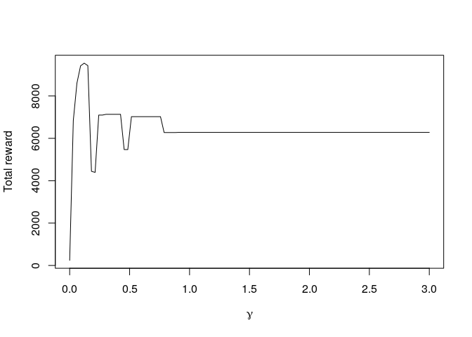
The relation between γ and the total accumulated reward looks somewhat strange, but it is important to realise that we are working with a single realisation of the task (as given in the rewards data frame). We are also always using the same random seed to increase the comparability between the different simulations. But that also means that the certain things, such as the initial random choice, are the same in each simulation. Anyway, for this particular realisation and random seed, the optimal value is γ = 0.121, which obtains a total reward of 9549.284. A proper evaluation of the optimal value of γ over many realisations of this task (with different means and rewards) requires a much more extensive simulation study. Perhaps we will do this in another blog post…

UCB

Simulating an RL agent with the UCB choice rule is much the same as previously, so we won’t need to ponder the code too much. One thing to note is the use of the which.is.max function from the nnet package, rather than the which.max function from base R. When there are multiple maxima, the latter function returns the index of the first element which reaches this maximum. This is one way to resolve a tie, but also rather arbitrary. The which.is.max resolves ties by randomly drawing an index from all elements which reach the maximum. I believe that this is a better solution for an RL agent, and hence I use this function.

library(nnet)
rl_ucb_sim <- function(rewards,m0,v0,sigma_xi_sq,sigma_epsilon_sq,beta) {
  nt <- nrow(rewards)
  no <- ncol(rewards)
  m <- matrix(m0,ncol=no,nrow=nt+1)
  v <- matrix(v0,ncol=no,nrow=nt+1)
  choice <- rep(0,nt)
  reward <- rep(0.0,nt)
  for(t in 1:nt) {
    # choose the option with the highest UCB, breaking ties at random
    choice[t] <- which.is.max(m[t,] + beta*sqrt(v[t,]) + sigma_xi_sq)
    reward[t] <- rewards[t,choice[t]]
    # Kalman updates:
    kt <- rep(0,4)
    kt[choice[t]] <- (v[t,choice[t]] + sigma_xi_sq)/(v[t,choice[t]] + sigma_xi_sq + sigma_epsilon_sq)
    m[t+1,] <- m[t,] + kt*(reward[t] - m[t,])
    v[t+1,] <- (1-kt)*(v[t,] + sigma_xi_sq)
  }
  return(list(m=m,v=v,choice=choice,reward=reward))
}

For our initial simulation, we will use a 95% confidence interval, corresponding to a choice of β = 1.96:

set.seed(123)
sim_ucb_196 <- rl_ucb_sim(rewards_mat,m0=0.0,v0=1000,sigma_xi_sq=16,sigma_epsilon_sq=16,beta=1.96)
plot_sim(sim_ucb_196)

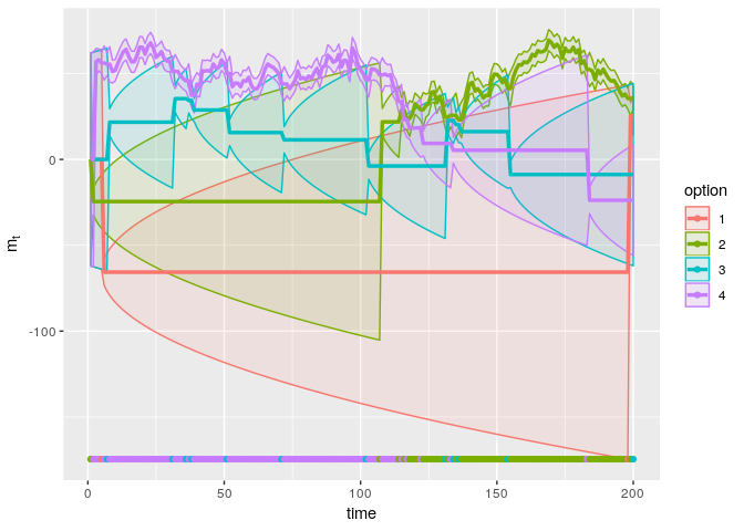
The UCB agent explores all options, and accumulates a total reward of 9037.143. The regret is 995.458. This is better than the two simulated softmax agents. As the plot shows, this agent explores more initially, allowing her to determine that option 4 is the best, but occasionally checking the second best option (option 3) whenever the upper confidence bound exceeds that of the preferred option (option 4).

If we choose a lower value of β, such as β = 1, exploration should be reduced:

set.seed(123)
sim_ucb_100 <- rl_ucb_sim(rewards_mat,m0=0.0,v0=1000,sigma_xi_sq=16,sigma_epsilon_sq=16,beta=1)
plot_sim(sim_ucb_100)

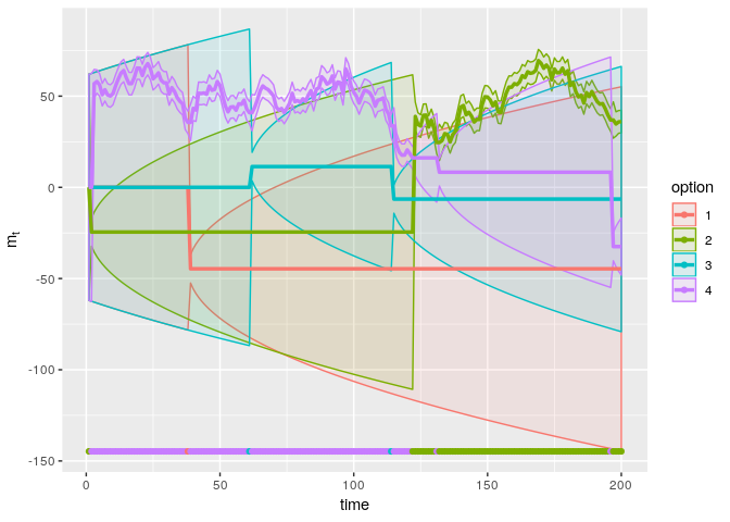
With this choice of β, the agent achieves a total reward of 9378.934, corresponding to a regret of 653.667. This is better than with β = 1.96, but again, it is important to realise that this evaluation is based on a single realisation of the task.

As performance depends on the choice of β, it is again interesting to see how the accumulated reward varies with different choices for β:

beta <- seq(0,3,length=100)
out <- rep(0,100)
for(i in 1:length(beta)) {
  set.seed(123)
  sim <- rl_ucb_sim(rewards_mat,m0=0.0,v0=1000,sigma_xi_sq=16,sigma_epsilon_sq=16,beta=beta[i])
  out[i] <- sum(sim$reward)
}
plot(beta,out,type="l",xlab=expression(beta),ylab="Total reward")

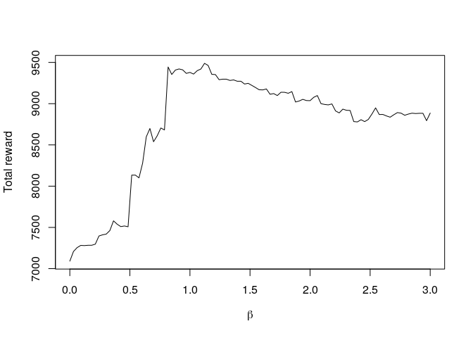
For this particular realisation of the task, the optimal value is β = 1.121, for which the total accumulated reward is 9488.857.

Thompson sampling

The code to simulate the RL agent with Thompson sampling is much the same as before. We use rnorm with a vector of different means and a vector of different standard deviations to draw samples from the four prior distributions of mean reward, and then use the which.is.max function again to pick the option with the highest value (in this case, it is extremely unlikely that multiple options have the same maximum sampled value, so we could have also used the which.max function).

rl_thompson_sim <- function(rewards,m0,v0,sigma_xi_sq,sigma_epsilon_sq) {
  nt <- nrow(rewards)
  no <- ncol(rewards)
  m <- matrix(m0,ncol=no,nrow=nt+1)
  v <- matrix(v0,ncol=no,nrow=nt+1)
  choice <- rep(0,nt)
  reward <- rep(0.0,nt)
  for(t in 1:nt) {
    # draw values from the prior distributions of the mean reward
    sim_r <- rnorm(4,mean=m[t,],sd=sqrt(v[t,] + sigma_xi_sq))
    # choose the option with the highest sampled value
    choice[t] <- which.is.max(sim_r)
    reward[t] <- rewards[t,choice[t]]
    # Kalman updates:
    kt <- rep(0,4)
    kt[choice[t]] <- (v[t,choice[t]] + sigma_xi_sq)/(v[t,choice[t]] + sigma_xi_sq + sigma_epsilon_sq)
    m[t+1,] <- m[t,] + kt*(reward[t] - m[t,])
    v[t+1,] <- (1-kt)*(v[t,] + sigma_xi_sq)
  }
  return(list(m=m,v=v,choice=choice,reward=reward))
}
set.seed(123)
sim_thompson <- rl_thompson_sim(rewards_mat,m0=0.0,v0=1000,sigma_xi_sq=16,sigma_epsilon_sq=16)
plot_sim(sim_thompson)

The Thompson agent explores all options and achieves a total reward of 8364.495. The regret is 1668.107. While this is worse than the UCB agent, the Thompson agent has no other parameters than those needed for the Kalman filter. As we have seen, the performance of the softmax and UCB agent depend on the value of γ and β respectively, and determining appropriate values for these is not trivial. For a randomly chosen value of β or γ, the Thompson sampling agent might perform better or worse than the UCB or softmax agent, respectively. Thus, we could determine the relatively performance of the Thompson sampling agent with the average performance of the UCB and softmax agents over a range of values of β and γ. Again, this should be based on a much more extensive simulation. Perhaps we will do so in another blog post.

Conclusion

In this post, I have introduced the restless bandit task, and the Kalman filter as a Bayesian model of learning the average value of (restless) bandits. The Kalman filter adjusts the learning rate to uncertainty and parameters of the environment, and as such can be viewed as a rational version of the delta-rule. Important characteristics of the Kalman filter in a bandit setting are that uncertainty and learning rate increase when a bandit hasn’t been tried for some time. The increase in learning rate allows inference to quickly catch up, while the increase in uncertainty will increase exploration when a choice rule is applied that takes uncertainty into account. I introduced three choice rules to balance exploration and exploitation: softmax, upper confidence bound (UCB), and Thompson sampling. While the softmax rule only considers the (estimated) value of options, and roughly chooses options according to their relative value, the UCB rule and Thompson sampling will both explore options more when they are more uncertain. While the performance of the softmax and UCB rule depends on the choice of crucial parameters (the “inverse temperature” γ for the softmax, and the “exploration bonus” β for the UCB), Thompson sampling does not require an additional parameter.

In the next post in this series, we will apply our understanding of the three models to fit them to behaviour from humans performing a restless bandit task. We will start with maximum likelihood estimation. In later posts, I aim to also cover Bayesian estimation.

References

Durbin, James, and Siem Jan Koopman. 2012. Time Series Analysis by State Space Methods. Oxford university press.

Gittins, John, Kevin Glazebrook, and Richard Weber. 2011. Multi-Armed Bandit Allocation Indices. John Wiley & Sons.

Kalman, R. E. 1960. “A New Approach to Linear Filtering and Prediction Problems.” Transactions of the American Society of Mechanical Engineers, Series D, Journal of Basic Engineering 82: 35–45.

Kalman, R. E., and R. S. Bucy. 1961. “New Results in Linear Filtering and Prediction Theory.” Transactions of the American Society of Mechanical Engineers, Series D, Journal of Basic Engineering 83: 95–108.

Speekenbrink, M., and E. Konstantinidis. 2015. “Uncertainty and Exploration in a Restless Bandit Problem.” Topics in Cognitive Science 7 (2): 351–67. doi:10.1111/tops.12145.

Sutton, Richard S., and Andrew G. Barto. 1998. Reinforcement Learning: An Introduction. Cambridge, MA, US: MIT Press.

Thompson, William R. 1933. “On the Likelihood that One Unknown Probability Exceeds Another in View of the Evidence of Two Samples.” Biometrika 25: 285–94. doi:10.2307/2332286.